How to Use INDEX and MATCH in Excel: Simple Guide

Before XLOOKUP, INDEX and MATCH was the best way to look up values in Excel. Unlike VLOOKUP, it can look up values to the left and to the right.

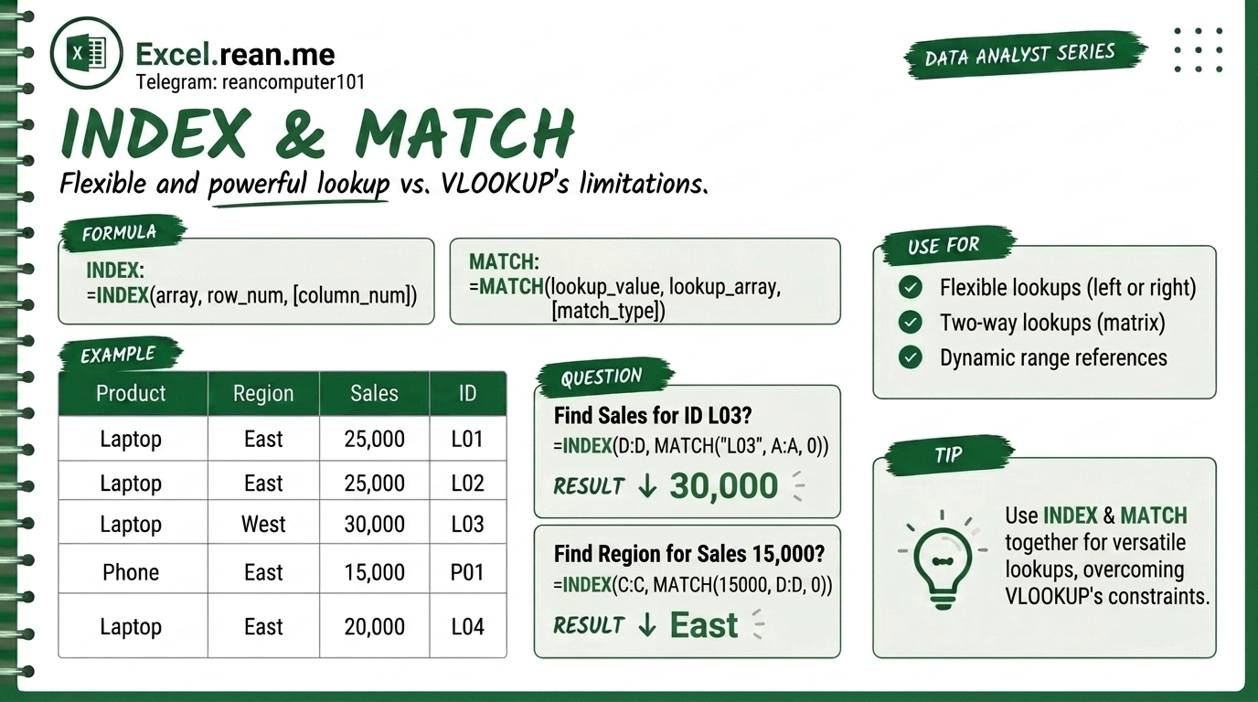
Why Use INDEX & MATCH?

• VLOOKUP can only look from left to right.
• INDEX and MATCH can look in any direction (left, right, up, down).

1. How the INDEX Formula Works

INDEX returns a cell value from a specific row and column position in a table.

=INDEX(array, row_num, [column_num])

• array: The group of cells to get your value from.
• row_num: The row number you want.
• column_num: The column number you want (Optional).

INDEX Video Tutorial (Khmer)

2. How the MATCH Formula Works

MATCH finds the position number of a value in a list.

=MATCH(lookup_value, lookup_range, match_type)

• lookup_value: The value you want to search for.
• lookup_range: The column or row to look in.
• match_type: Use 0 for an exact match.

MATCH Video Tutorial (Khmer)

3. Combining INDEX and MATCH Together

Put MATCH inside INDEX to find a value automatically based on a search term:

=INDEX(C2:C100, MATCH("Product A", A2:A100, 0))

This finds "Product A" in column A, gets its row number, and returns the matching value from column C.

Example #1 INDEX & MATCH Video Tutorial in Khmer

Example #2 INDEX & MATCH Video Tutorial in Khmer

4. Two-Way (2D Grid) Lookups

You can combine a row MATCH and a column MATCH inside INDEX to look up data in a 2D matrix:

=INDEX(B2:G10, MATCH("Sales", A2:A10, 0), MATCH("Q3", B1:G1, 0))