How to use MIN vs MAX and SMALL vs LARGE Functions in Excel (Video in Khmer)

Hello everyone! In today's video tutorial, you will learn how to use MIN, MAX, SMALL, and LARGE functions in Microsoft Excel with simple step-by-step examples.

These statistical functions allow you to quickly find the highest, lowest, 2nd highest, or 3rd lowest values in your dataset.

📚 Related Tutorial: Want to learn keyboard shortcuts? Check out our guide on Learn All Excel Keyboard Shortcuts!

📊 Quick Comparison Table

Function	What It Finds	Formula Syntax	Example Output
`MIN`	Absolute lowest value	`=MIN(range)`	`=MIN(A1:A5)` -> `20`
`MAX`	Absolute highest value	`=MAX(range)`	`=MAX(A1:A5)` -> `95`
`SMALL`	k-th lowest value	`=SMALL(array, k)`	`=SMALL(A1:A5, 2)` -> `50` (2nd lowest)
`LARGE`	k-th highest value	`=LARGE(array, k)`	`=LARGE(A1:A5, 2)` -> `85` (2nd highest)

🛠️ 1. MIN and MAX Functions

MIN: Returns the smallest number in a list of values.
MAX: Returns the largest number in a list of values.

Formula Syntax:

=MIN(number1, [number2], ...)
=MAX(number1, [number2], ...)

Example:

Given test scores in cells A1:A5: [50, 85, 20, 95, 70]

Find lowest score: =MIN(A1:A5) -> 20
Find highest score: =MAX(A1:A5) -> 95

📚 Related Tutorial: Learn more foundational formulas in our guide on Top 15 Basic Excel Formulas for Beginners ↗!

🛠️ 2. SMALL and LARGE Functions

Unlike MIN and MAX which only find absolute extreme values, SMALL and LARGE let you specify position ranking (k).

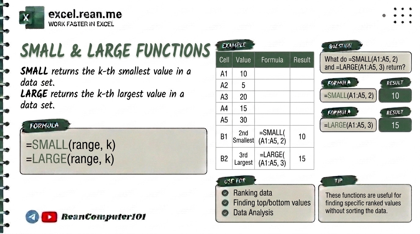
Formula Syntax:

=SMALL(array, k)
=LARGE(array, k)

array: The cell range of numbers.
k: The position rank (1 for 1st, 2 for 2nd, 3 for 3rd, etc.).

Example:

Given test scores in cells A1:A5: [50, 85, 20, 95, 70] (sorted: 20, 50, 70, 85, 95)

Find 2nd lowest score: =SMALL(A1:A5, 2) -> 50
Find 3rd lowest score: =SMALL(A1:A5, 3) -> 70
Find 2nd highest score (Runner-up): =LARGE(A1:A5, 2) -> 85
Find 3rd highest score: =LARGE(A1:A5, 3) -> 70

💡 Pro Tips

Calculate Sum of Top 3 Values: Combine SUM and LARGE to add up your top 3 sales figures:
```
=SUM(LARGE(A1:A10, {1,2,3}))
```
SMALL(..., 1) vs MIN(...): =SMALL(A1:A10, 1) gives the exact same result as =MIN(A1:A10). Similarly, =LARGE(A1:A10, 1) gives the exact same result as =MAX(A1:A10).
Avoid #NUM! Error: Make sure k is a positive integer between 1 and the total count of numbers in your array. If k exceeds the data count, Excel returns a #NUM! error.